R | spatial data: points in polygon with San Francisco crime data

The San Francisco crime dataset hosted by SF OpenData has provided me a good opportunities to test out some of R’s spatial analysis libraries. All the coordinate information has already been included so we don’t need to worry about geocoding ourselves. Kaggle has divided the entire databset it into train and test sub-datasets for its knowledge-based San Francisco Crime Classification competition. The train set is all what I am going to use here. A good exercise to work on would be to group all the observations into geographical areas using all the available spatial information. The dataset has already group everyone into police department districts. So we need to find something else. Zipcode might be something worth trying. To get the geographical data for our purpose here, we can again go to Open SF Data and download the shapefile pack. Now unzip the downloaded pack and save all the files into the working directory. I have saved them into a new folder called sf_zipcode. We can then load the shapefile into r using rgdal library.

library(rgdal)

sf <- readOGR(dsn = "sf_zipcode", layer = "sfzipcodes")
sf <- spTransform(sf, CRS("+proj=longlat +datum=WGS84"))

As above the file is loaded using the readOGR() function. Argument dsn specify which folder to look in, so if you same the file in your working directory root then this should just be dsn = ".". Then layer specify the .shp file name, without the extention. Note that this will also read in .prj file, which contains the projection information for our spatial dataset here. For those without knowledge in Geodesy (like myself) this might be the tricky bit. The default coordinate system in this shapefile belongs to something called Lambert Conformal Conic, which is not compatible with the standard WGS84 system used in our crime dataset’s latitude and lontitude columns. To transform it to the WGS84 system we just need to run the following:

sf <- spTransform(sf, CRS("+proj=longlat +datum=WGS84"))

Now that we have right coordinate system for both the base SF map and crime dataset, we can do some basic plot with both of them. Below is just a example using r version of the famous leaflet toolset. I will also load dplyr library here, at the moment just for its %>% operator but I will use a bit more of it later.

library(leaflet)
library(dplyr)

leaflet(sf) %>%
  addProviderTiles("CartoDB.Positron") %>%
  addPolygons() %>%
  addMarkers(lng <- cri[cri$Category == "GAMBLING",c("X")], lat = cri[cri$Category == "GAMBLING",c("Y")]) %>%
  setView(lng <- cri[cri$Category == "GAMBLING",c("X")][1], lat = cri[cri$Category == "GAMBLING",c("Y")][1],zoom = 12)

This should plots the below interactive map that looks like below: We can now prepare the train dataset for our points-in-polygons operation. To do this we first need to construct all the coordinates in train set into a SpatialPoints formation, where coordinates are saved in pairs. Just run the following:

cri.cord <- data.frame(X = cri$X, Y = cri$Y)
cri.cord <- SpatialPoints(cri.cord)
proj4string(cri.cord) <- proj4string(sf)

sf.poly <- sf@polygons

Function proj4string() is used to ensure the SpatialPoints item here knows it is using the same coordinate reference system (CRS as we have already seen in during spTransform) as sf. In the last line we have also extracted the polygons component from the overall sf spatial dataset. Now we are ready to perform the points-in-polygons operation, below is a customised function for this purpose.

getPostcode <- function(SP_unit,row.n){
  for(i in 1:length(sf.poly)){
    a <- SpatialPolygons(sf.poly[i])
    proj4string(a) <- proj4string(cri.cord)
    b <- over(SP_unit[row.n],a)
    if(!is.na(b)){
      return(sf$ZIP_CODE[i])
    }
  }
}

This function takes two inputs - the SpatialPoints object conaining multiple pairs of coordinates and the row number specifying which pair to use. This will loop through all 25 polygons stored in sf.poly, corresponding to the 25 zipcode areas, and check if the coordinate belongs in the polygon though the over() function. After it finds a match it will then return the zipcode number as output. Now we just need another loop to go thorugh each row in cri.cord and find all the zipcodes. We can do this through the following:

train_postcode = c()
total <- nrow(cri)

pb <- winProgressBar(title="Example progress bar", label="0% done", min=0, max=total, initial=0)

for(i in length(train_postcode)+1:total){
  train_postcode[i] <- if(!is.null(getPostcode(cri.cord,i))){
    getPostcode(cri.cord,i)
  } else {
    ""
  }
  info <- sprintf("%f%% done", (i/total)*100)
  setWinProgressBar(pb, i/total*100, label=info)
}
close(pb)

Note that this piece of code uses a basic for loop, thus to go through all 800k of rows it would normally take more than 10 hours to finish. This is why I have included a winProgressBar just so I know how much has been done. One potential solution for this performance issue would be to use a parallel processing facility provided by libraries like foreach. I do believe there are ways to make significant improvement to this, and I am open to any advise on this. Now that we have a vector of all the zipcode information we can plug this back into our master crime dataset, and do some map plots related to zipcode . Below is just a very basic example - a all time crime density in each post area.

cri <- data.frame(cri,Zipcode = train_Zipcode)

cri_zip <- cri %>%
  group_by(Zipcode) %>%
  summarise(Number_of_Crimes = n()) %>%
  data.frame()

cri_zip <- cri_zip[!cri_zip$Zipcode == "",]
sf@data <- merge(sf@data,cri_zip,by.x="ZIP_CODE",by.y="Zipcode")

pal <- colorNumeric(palette = "Reds", domain = sf$Number_of_Crimes)

m <- leaflet(sf) %>%
  addProviderTiles("CartoDB.Positron") %>%
  addPolygons(stroke = F, color = ~pal(Number_of_Crimes)) %>%
  addLegend("bottomright", pal = pal, values = ~Number_of_Crimes,
            title = "Number of crimes ('0)",
            opacity = 1
  )

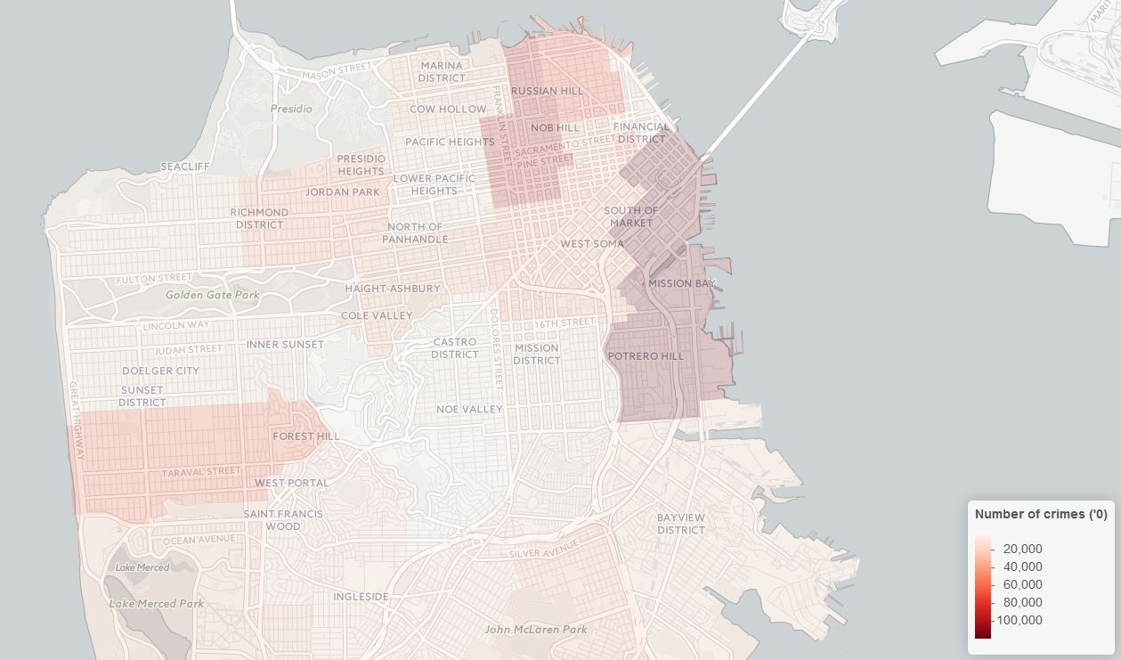Hope this provides a bit of idea on how to match some coordinates to areas on a map using R’s spatial analysis tools. You can find a complete version of all the codes and datasets used in this post at my github page, including the completed zipcode for kaggle’s train dataset so to save your a few hours time running the loop yourself.